Coupling Groups, Copulas and Variable Reordering
This guide explains how PAL manages dependencies between stochastic variables. It covers three interconnected concepts:
Coupling Groups — automatic tracking of related variables
Copulas — creating dependency structures between variables
Variable Reordering — how copulas work under the hood
A runnable version of all examples below is available at
examples/example_couplings_and_copulas.py.
1. Coupling Groups
What Is a Coupling Group?
Every StochasticScalar in PAL belongs to a coupling group — a
set of variables that are linked by computation. When you create an
independent variable, it gets its own coupling group. When you combine
variables in arithmetic, their coupling groups merge.
from pal import config, distributions, set_random_seed

config.n_sims = 10_000
set_random_seed(42)

motor = distributions.LogNormal(mu=14, sigma=0.5).generate()
prop = distributions.LogNormal(mu=15, sigma=0.8).generate()

# Each starts in its own group
motor.coupled_variable_group is prop.coupled_variable_group
# => False
When variables are combined, they become coupled:
total = motor + prop

# Now all three share the same coupling group
motor.coupled_variable_group is prop.coupled_variable_group
# => True

len(motor.coupled_variable_group)
# => 3
Derived variables also join automatically:
motor_with_expenses = motor * 1.1

motor_with_expenses.coupled_variable_group is motor.coupled_variable_group
# => True

len(motor.coupled_variable_group)
# => 4
Why Coupling Groups Matter
Coupling groups solve a critical problem: when a copula reorders one variable’s simulations, all related variables must be reordered in exactly the same way to preserve their mathematical relationships.
Consider this scenario:
set_random_seed(42)
loss_a = distributions.LogNormal(mu=14, sigma=0.5).generate()
loss_b = distributions.LogNormal(mu=15, sigma=0.8).generate()

# Derive a variable from loss_a
loss_a_expenses = loss_a * 1.15  # 15% expense loading
Before any copula, loss_a and loss_a_expenses have a perfect 1.15×
relationship because simulation i of both variables corresponds to the
same underlying scenario:
loss_a first 5:          [1751476. 1113583. 2057538. 1557236.  622980.]
loss_a_expenses first 5: [2014197. 1280620. 2366169. 1790821.  716427.]
Ratio:                   [1.15 1.15 1.15 1.15 1.15]
Now apply a copula to correlate loss_a with loss_b:
from pal import copulas

copulas.GaussianCopula(
    [[1.0, 0.7], [0.7, 1.0]]
).apply([loss_a, loss_b])
After the copula reorders loss_a, the 1.15× ratio is preserved:
Ratio (still 1.15!): [1.15 1.15 1.15 1.15 1.15]
This works because PAL’s coupling group system automatically reordered
loss_a_expenses with the same permutation as loss_a.
Without coupling groups, loss_a_expenses would retain its original
ordering while loss_a was shuffled, breaking the 1.15× relationship
and producing nonsensical results.
2. Copulas
A copula defines a dependency structure (correlation pattern) between random variables. PAL provides several copula families, each producing different patterns of dependence, especially in the tails.
Available Copula Types
Family |
Class |
Key Parameters |
Tail Dependence |
|---|---|---|---|
Elliptical |
|||
Gaussian |
|
Correlation matrix |
None |
Student’s T |
|
Correlation matrix, |
Symmetric |
Archimedean |
|||
Gumbel |
|
|
Upper |
Clayton |
|
|
Lower |
Frank |
|
|
None |
Joe |
|
|
Upper |
Extreme value |
|||
MM1 |
|
|
Upper |
Galambos |
|
|
Upper |
Hüsler-Reiss |
|
|
Upper |
Extremal T |
|
|
Upper |
Other |
|||
Plackett |
|
|
None |
Elliptical copulas (Gaussian, Student’s T) accept a full correlation matrix and naturally support any number of dimensions.
Archimedean copulas (Gumbel, Clayton, Frank, Joe) take a single
theta parameter and the dimension n.
Extreme value copulas (MM1, Galambos, Hüsler-Reiss, Extremal T) model upper tail dependence and are suited for modelling joint extreme events. They have varying parameterisations — see the API docs for details.
Plackett copula is a bivariate copula controlled by a single
parameter delta that can model both positive and negative dependence.
Comparing Copula Types
from pal import config, copulas, distributions, set_random_seed
import numpy as np

config.n_sims = 10_000
Independent (no copula)
set_random_seed(42)
x = distributions.LogNormal(mu=10, sigma=1.0).generate()
y = distributions.LogNormal(mu=10, sigma=1.0).generate()

np.corrcoef(x.ranks.values, y.ranks.values)[0, 1]
# => -0.0034  (approximately zero)
Gaussian Copula
set_random_seed(42)
x = distributions.LogNormal(mu=10, sigma=1.0).generate()
y = distributions.LogNormal(mu=10, sigma=1.0).generate()
copulas.GaussianCopula([[1.0, 0.8], [0.8, 1.0]]).apply([x, y])

np.corrcoef(x.ranks.values, y.ranks.values)[0, 1]
# => 0.7853
Gumbel Copula (upper tail dependence)
set_random_seed(42)
x = distributions.LogNormal(mu=10, sigma=1.0).generate()
y = distributions.LogNormal(mu=10, sigma=1.0).generate()
copulas.GumbelCopula(theta=3.0).apply([x, y])

np.corrcoef(x.ranks.values, y.ranks.values)[0, 1]
# => 0.8465
Variables jointly tend to be large together — important for modelling joint catastrophic losses.
Clayton Copula (lower tail dependence)
set_random_seed(42)
x = distributions.LogNormal(mu=10, sigma=1.0).generate()
y = distributions.LogNormal(mu=10, sigma=1.0).generate()
copulas.ClaytonCopula(theta=4.0).apply([x, y])

np.corrcoef(x.ranks.values, y.ranks.values)[0, 1]
# => 0.8479
Variables jointly tend to be small together — dependence is concentrated in the lower tail.
Student’s T Copula (symmetric tail dependence)
set_random_seed(42)
x = distributions.LogNormal(mu=10, sigma=1.0).generate()
y = distributions.LogNormal(mu=10, sigma=1.0).generate()
copulas.StudentsTCopula(
    [[1.0, 0.7], [0.7, 1.0]], dof=3
).apply([x, y])

np.corrcoef(x.ranks.values, y.ranks.values)[0, 1]
# => 0.6658
Like the Gaussian copula but with symmetric tail dependence — extreme values are more likely to co-occur. The lower the degrees of freedom, the stronger the tail dependence.
Scatter Plots — Rank Space
The best way to understand how copulas differ is to plot the variables in rank space (plotting the ranks rather than the raw values). This removes the effect of the marginal distributions and isolates the dependency structure.
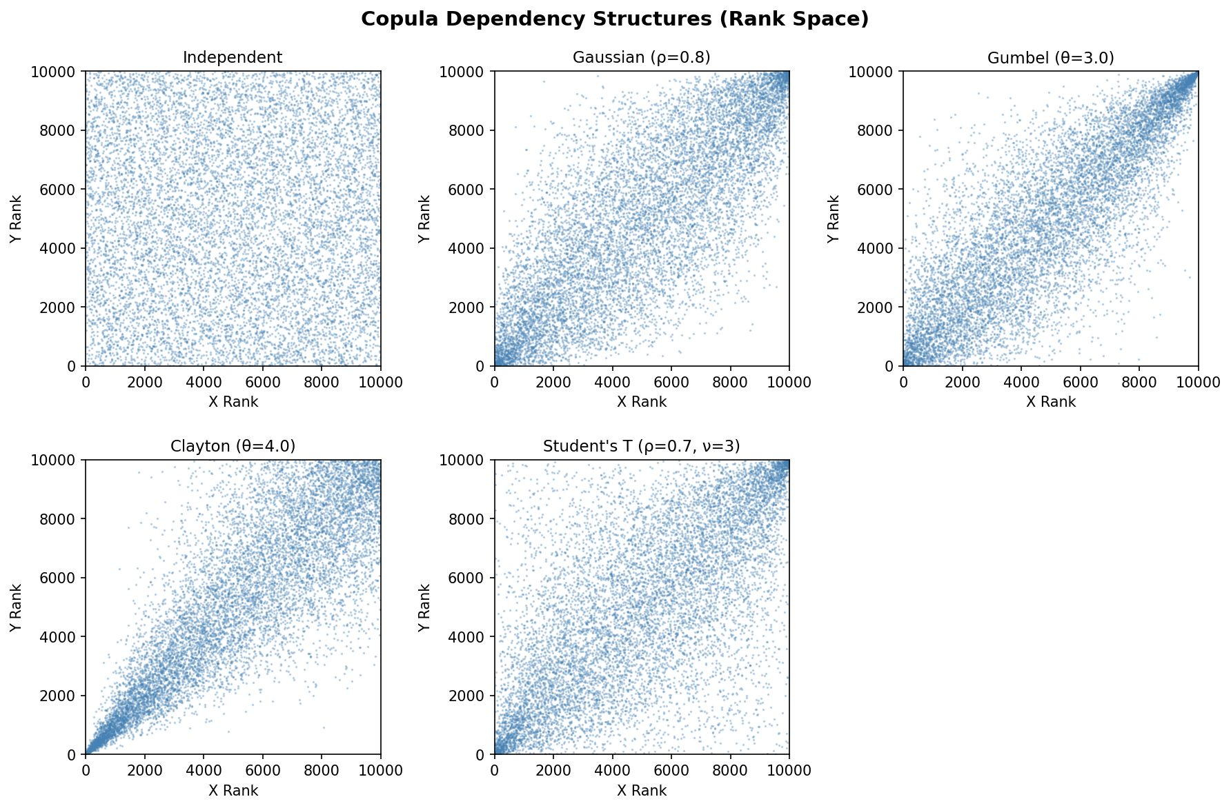
Independent: uniform scatter with no pattern
Gaussian: elliptical concentration along the diagonal
Gumbel: strong clustering in the upper-right corner (upper tail)
Clayton: strong clustering in the lower-left corner (lower tail)
Student’s T: similar to Gaussian but with heavier concentration in both corners (both tails)
The interactive version of this chart (with plotly) is available in
examples/example_couplings_and_copulas.ipynb.
3. Variable Reordering
How apply() Works
When you call copula.apply([var_x, var_y]), PAL performs these steps:
Generate copula samples: The copula creates correlated uniform random variables with the desired dependency structure.
Compute rank indices: For each copula sample, compute the rank ordering (which simulation should be 1st, 2nd, 3rd, etc.).
Reorder simulations: Rearrange each variable’s simulations so their ranks match the copula’s rank structure.
Preserve marginals: The same set of values is retained — only their ordering changes.
Merge coupling groups: All input variables (and their coupled variables) are merged into a single coupling group.
Seeing Reordering in Action
To make the reordering concrete, here is a small example with only 8 simulations. We can see exactly which values move where:
config.n_sims = 8
set_random_seed(42)

x = distributions.Normal(0, 1).generate()
y = distributions.Normal(0, 1).generate()
Before the copula, X and Y have unrelated orderings:
         Sim:    0      1      2      3      4      5      6      7
  X values:  [ 0.752, -0.154,  1.074,  0.517, -1.315,  1.971,  0.710,  0.793]
  Y values:  [-1.135, -0.125, -0.330,  1.452,  0.369,  0.926, -0.142, -0.748]
  X ranks:   [    4,      1,      6,      2,      0,      7,      3,      5]
  Y ranks:   [    0,      4,      2,      7,      5,      6,      3,      1]
Notice that X and Y ranks are unrelated — when X is high (rank 7 in sim 5), Y has rank 6. When X is low (rank 0 in sim 4), Y has rank 5.
copulas.GaussianCopula([[1, 0.9], [0.9, 1]]).apply([x, y])
After the copula, the Y values have been shuffled so their ranks align with X’s ranks:
         Sim:    0      1      2      3      4      5      6      7
  X values:  [ 0.752, -0.154,  1.074,  0.517, -1.315,  1.971,  0.710,  0.793]
  Y values:  [-0.125, -0.748,  0.926, -0.142, -1.135,  1.452, -0.330,  0.369]
  X ranks:   [    4,      1,      6,      2,      0,      7,      3,      5]
  Y ranks:   [    4,      1,      6,      3,      0,      7,      2,      5]
Key observations:
X values are unchanged — the same 8 numbers in the same positions
Y values are the same set of numbers, but reordered — e.g. the value
1.452moved from sim 3 to sim 5Ranks now nearly match: when X has rank 7 (sim 5), Y also has rank 7. When X has rank 0 (sim 4), Y also has rank 0
Sorted values are identical before and after:
np.allclose(sorted(x.values), sorted_x) # => TrueRank correlation jumped to 0.9762 (from ~0)
This is the fundamental mechanism: copula application is a permutation, not a transformation.
Marginal Preservation
A critical property of copula application is that marginal distributions are exactly preserved. The same values exist before and after — only their ordering changes:
config.n_sims = 10_000
set_random_seed(42)
var_x = distributions.Normal(0, 1).generate()
var_y = distributions.Normal(0, 1).generate()

sorted_x = np.sort(var_x.values)
sorted_y = np.sort(var_y.values)

copulas.GaussianCopula(
    [[1.0, 0.9], [0.9, 1.0]]
).apply([var_x, var_y])

# Marginals are unchanged
np.allclose(np.sort(var_x.values), sorted_x)  # => True
np.allclose(np.sort(var_y.values), sorted_y)  # => True

# But now correlated
np.corrcoef(var_x.ranks.values, var_y.ranks.values)[0, 1]
# => 0.8903
Reordering Across a Chain of Derived Variables
Coupling groups enable transitive reordering across chains of derived variables:
set_random_seed(42)

base_loss = distributions.LogNormal(mu=14, sigma=0.5).generate()
gross_loss = base_loss * 1.0
expense_loaded = gross_loss * 1.10
tax = expense_loaded * 0.21
net_loss = expense_loaded - tax

# All 5 variables share one coupling group
len(base_loss.coupled_variable_group)
# => 5
When a copula is applied to base_loss and an independent variable,
every variable in the chain is reordered together:
cat_loss = distributions.LogNormal(mu=16, sigma=1.2).generate()
copulas.GumbelCopula(theta=1.5).apply(
    [base_loss, cat_loss]
)

# All ratios are preserved
gross_loss.values[:3] / base_loss.values[:3]
# => [1. 1. 1.]

expense_loaded.values[:3] / gross_loss.values[:3]
# => [1.1 1.1 1.1]

tax.values[:3] / expense_loaded.values[:3]
# => [0.21 0.21 0.21]
4. Multivariate Copulas
Elliptical copulas naturally extend to any number of dimensions. Here is an example correlating 4 lines of business:
set_random_seed(42)

lobs = {
    "Motor": distributions.LogNormal(mu=14, sigma=0.4).generate(),
    "Property": distributions.LogNormal(mu=15, sigma=0.6).generate(),
    "Liability": distributions.LogNormal(mu=13, sigma=0.5).generate(),
    "Marine": distributions.LogNormal(mu=12, sigma=0.7).generate(),
}

corr_matrix = [
    [1.0, 0.6, 0.3, 0.2],
    [0.6, 1.0, 0.4, 0.3],
    [0.3, 0.4, 1.0, 0.5],
    [0.2, 0.3, 0.5, 1.0],
]

copulas.GaussianCopula(corr_matrix).apply(list(lobs.values()))
The resulting rank correlations closely match the input:
                Motor    Property   Liability      Marine
   Motor        1.000       0.578       0.264       0.177
   Property     0.578       1.000       0.361       0.261
   Liability    0.264       0.361       1.000       0.479
   Marine       0.177       0.261       0.479       1.000
Compare with input: [0.6, 0.3, 0.2], [0.4, 0.3], [0.5] — the rank
correlations are close but not exact due to finite sample size
(10,000 simulations).
To be completely precise, we should compare the rank correlation to the Spearman’s :math:\rho_S of the Gaussian copula, which is related to the underlying correlation parameter :math:r by:
.. math::
\rho_S = \frac{6}{\pi}\asin\left(\frac{r}{2}\right)
5. generate() vs apply()
Copulas have two main methods:
generate() — Create New Samples
Returns correlated uniform [0, 1] samples. Use this when you want
raw copula samples to feed into inverse CDF transforms manually:
samples = copulas.GaussianCopula(
    [[1.0, 0.8], [0.8, 1.0]]
).generate()

samples[0].mean()  # => ~0.5 (uniform)
samples[1].mean()  # => ~0.5 (uniform)
apply() — Reorder Existing Variables
Reorders existing StochasticScalar variables to match the copula’s
dependency structure. This is the most common workflow:
v1 = distributions.Gamma(alpha=5, theta=1000).generate()
v2 = distributions.Pareto(shape=2, scale=10000).generate()

copulas.GaussianCopula(
    [[1.0, 0.8], [0.8, 1.0]]
).apply([v1, v2])

# Means unchanged - only the ordering changed
# Rank correlation: 0.7867
Key difference: generate() creates new data; apply() restructures
existing data. In most actuarial models, you’ll use apply() because
you’ve already generated variables from their marginal distributions and
want to impose a dependency structure.
6. Frequency-Severity Models with Copulas
In actuarial modelling, losses are often represented as compound
distributions using FrequencySeverityModel. After generating
event-level simulations, you aggregate them to get simulation-level
totals, then use copulas to impose dependencies between lines of
business.
Two Lines of Business
from pal.frequency_severity import FrequencySeverityModel

config.n_sims = 10_000
set_random_seed(42)

# Motor: 50 claims/year, LogNormal severity
motor_model = FrequencySeverityModel(
    freq_dist=distributions.Poisson(mean=50),
    sev_dist=distributions.LogNormal(mu=10, sigma=1.5),
)
motor_events = motor_model.generate()

# Property: 20 claims/year, Pareto severity
property_model = FrequencySeverityModel(
    freq_dist=distributions.Poisson(mean=20),
    sev_dist=distributions.Pareto(shape=2.5, scale=50_000),
)
property_events = property_model.generate()

# Aggregate to simulation-level totals
motor_agg = motor_events.aggregate()
property_agg = property_events.aggregate()
Before the copula, the two lines are independent:
Before copula:
  Motor aggregate mean:         3,373,050
  Property aggregate mean:      1,664,453
  Rank correlation:               -0.0069
Now apply a Gaussian copula with ρ=0.6 (both lines worsen in the same economic environment):
copulas.GaussianCopula(
    [[1, 0.6], [0.6, 1]]
).apply([motor_agg, property_agg])
After the copula, losses are correlated but marginals are preserved:
After Gaussian copula (rho=0.6):
  Motor aggregate mean:         3,373,050
  Property aggregate mean:      1,664,453
  Rank correlation:                0.5780

Combined portfolio:
  Mean:                         5,037,503
  Std:                          1,744,284
  99.5th percentile:           12,192,519
The means are identical before and after — only the joint behaviour changed. The 99.5th percentile of the combined portfolio reflects the positive dependence: bad years for motor tend to also be bad years for property.
Coupling with Catastrophe Losses
You can also use copulas to link frequency-severity aggregate losses
with standalone catastrophe variables. Because aggregate() and
occurrence() return StochasticScalar objects that share a coupling
group with the underlying events, reordering the aggregate
automatically reorders the max-event loss too:
set_random_seed(42)

model = FrequencySeverityModel(
    freq_dist=distributions.Poisson(mean=30),
    sev_dist=distributions.LogNormal(mu=10, sigma=1.5),
)
events = model.generate()

agg_loss = events.aggregate()   # total loss per sim
max_loss = events.occurrence()  # largest single event per sim

cat_loss = distributions.LogNormal(mu=16, sigma=1.2).generate()

copulas.GumbelCopula(theta=2.0).apply(
    [agg_loss, cat_loss]
)
The Gumbel copula introduces upper tail dependence — years with high attritional losses also tend to have high catastrophe losses:
After Gumbel copula (theta=2.0):
  Agg loss mean:          2,022,548
  Max event mean:           637,503
  Cat loss mean:         18,398,184
  Rank corr (agg-cat):       0.6874
  Rank corr (max-cat):       0.5818
Note that the max-event loss is also correlated with the catastrophe
loss (rank corr 0.58) even though the copula was only applied to the
aggregate. This is because aggregate() and occurrence() share a
coupling group with the underlying FreqSevSims events.
Important Constraints
Variables must be independent before
apply(): You cannot apply a copula to variables that are already coupled (i.e., in the same coupling group). PAL raises aValueErrorif you try.Coupling is permanent: Once variables are coupled (either through arithmetic or copula application), they remain in the same coupling group for the rest of the simulation.
Order matters: The order of variables in the list passed to
apply()must match the order of dimensions in the copula’s correlation matrix.
References
Nelsen, R. B. (2006). An Introduction to Copulas, 2nd ed. Springer. — The standard textbook on copula theory; covers all major families, properties, and constructions.
McNeil, A. J., Frey, R. & Embrechts, P. (2015). Quantitative Risk Management: Concepts, Techniques and Tools, 2nd ed. Princeton University Press. — Chapters 7–8 give an accessible treatment of copulas in a risk-management context.
Iman, R. L. & Conover, W. J. (1982). “A distribution-free approach to inducing rank correlation among input variables.” Communications in Statistics — Simulation and Computation, 11(3), 311–334. — The original rank-reordering algorithm used by PAL’s
apply()method.Joe, H. (2014). Dependence Modeling with Copulas. CRC Press. — Comprehensive reference covering Archimedean, elliptical, and extreme-value copula families.
Embrechts, P., Lindskog, F. & McNeil, A. (2003). “Modelling dependence with copulas and applications to risk management.” In Handbook of Heavy Tailed Distributions in Finance, Elsevier. — Practical guide to choosing and calibrating copulas for insurance and finance applications.